Land or Water? - numpy with large datasets
Let’s look at how we handle large data sets in numpy. As an example, we’ll take a world map at 1km resolution per pixel.
Dataset
The example data comes from (the now closed) http://www.landcover.org/data/landcover/. The University of Maryland Department of Geography generated this global land cover classification collection in 1998. Imagery from the AVHRR satellites acquired between 1981 and 1994 were analyzed to classify the world’s surface into fourteen land cover types at a resolution of 1 km 1 .
Download
First, let’s get all files we need, then we’ll discuss them afterwards. Create a new empty directory to work in, and…
Download landcover.zip and extract the data file from it. It is called
gl-latlong-1km-landcover.bsqand should be 933120000 bytes big. Put the unzipped data file in your working directory. This is a raw binary file of data, with no internal description of how we can interpret it. Nowadays, one would use a self-describing format such as NetCDF for this kind of geographical data.The data format is described in a separate file
gl0500bs.txt(click to download).Information Image Size: 43200 Pixels 21600 Lines Quantization: 8-bit unsigned integer Output Georeferenced Units: LONG/LAT E019 Projection: Geographic (geodetic) Earth Ellipsoid: Sphere, rad 6370997 m Upper Left Corner: 180d00'00.00" W Lon 90d00'00.00" N Lat Lower Right Corner: 180d00'00.00" E Lon 90d00'00.00" S Lat Pixel Size (in Degrees): 0.00833 Lon 0.00833 Lat (Equivalent Deg,Min,Sec): 0d00'30.00"0d00'30.00" UpLeftX: -180 UpLeftY: 90 LoRightX: 180 LoRightY: -90
We’ll make sense of it later. For now, let’s note the first 2 lines: it’s meant to be an image of 21600 lines with 43200 pixels. And the values are stored as 8-bit unsigned integer.
The possible integer values go from 0 to 13, as we can see in the encoding of the land types mentioned on the project’s website:
landcover_legend.png(click to download)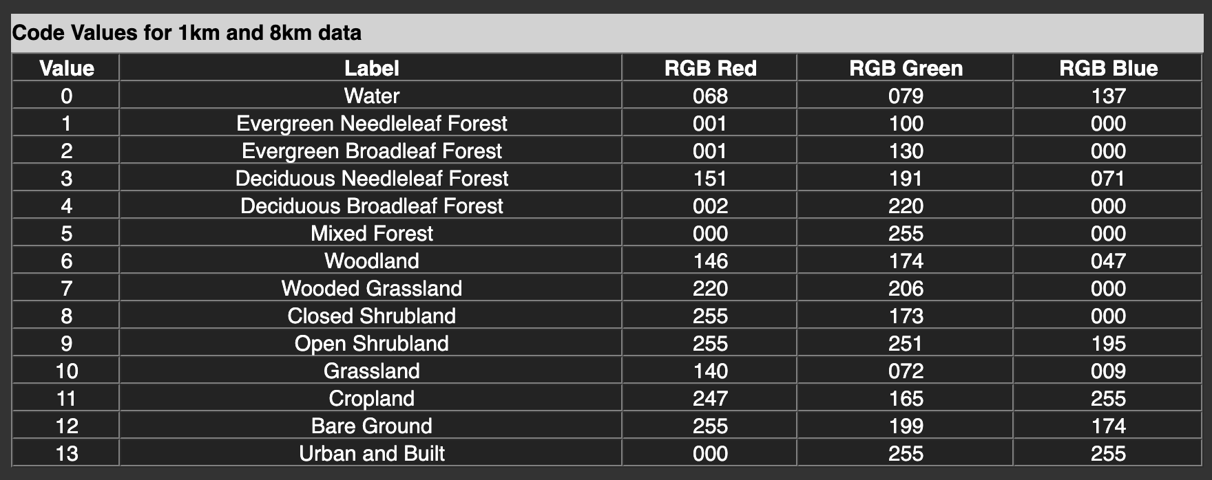
Making sense of it
What is actually in the data file? A search for “numpy load binary data” suggests
numpy.fromfile. Let’s try it:
import numpy as np
data = np.fromfile('gl-latlong-1km-landcover.bsq')

print('data', data)
print('minmax', data.min(), data.max())
print('shape', data.shape)
We get:
   data [0.00000000e+000 0.00000000e+000 0.00000000e+000 ... 1.22416778e-250
1.22416778e-250 1.22416778e-250]
   minmax 0.0 8.309872195179385e-246
   shape (116640000,)
The values here make no sense. What has gone wrong? We were expecting integer values in the data file, but got very small float values instead. Also, from a file of size 933120000, we only got 116640000 values. We must be misinterpreting the binary data.
Let’s look at the documentation of
np.fromfile
We see that there is a dtype parameter we can specify, to determine the data type.
By default it is float, which in Python is a 64-bit data type. So we are taking 64 bits
from the file and interpreting them as a float number. Instead, the description told
us it was 8-bit unsigned integer. In numpy, this is represented as uint8
(see numpy basic types)
Let’s try to specify this explicitly:
import numpy as np
data = np.fromfile('gl-latlong-1km-landcover.bsq', dtype='uint8')

print('data', data)
print('minmax', data.min(), data.max())
print('shape', data.shape)
The result is a lot better:
data [ 0  0  0 ... 12 12 12]
minmax 0 13
shape (933120000,)
We see that the values are integers, and they go from 0 to 13 like we expect. Only the shape is still strange. It should be 2-dimensional with 43200 pixels and 21600 lines. Instead, we have a one-dimensional long array with 933 million values. But \(43200\times 21600=933120000\)!
Let’s reshape the array into the right form:
data = np.fromfile('gl-latlong-1km-landcover.bsq', dtype='uint8')
data = data.reshape(21600, 43200)
Now the output is the right shape:
data [[ 0  0  0 ...  0  0  0]
 [ 0  0  0 ...  0  0  0]
 [ 0  0  0 ...  0  0  0]
 ...
 [12 12 12 ... 12 12 12]
 [12 12 12 ... 12 12 12]
 [12 12 12 ... 12 12 12]]
 minmax 0 13
 shape (21600, 43200)
Each position in the array approximately corresponds to a 1km x 1km square on Earth. The value at that position represents the dominant landcover.
Visualisation
Remember that we can use plt.imshow() to look at 2-dimensional arrays. Let’s
try that here. Viewing almost 1GB of data will be very resource-intensive. So
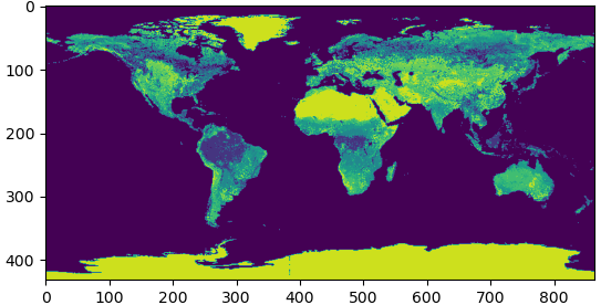
let’s do a subsample of the data. We go from beginning to end in steps of 50: ::50.
This will reduce the data size for plotting by \(50\times 50=2500\) to approximately
400kB:
viz_data = data[::50, ::50]

import matplotlib.pyplot as plt
plt.imshow(viz_data)
plt.show()
The result looks promising:
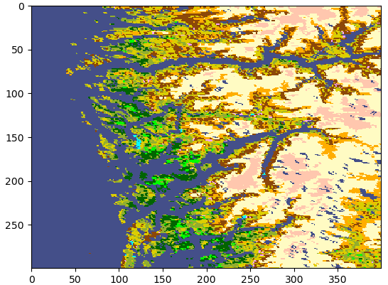
We can also use the original data set, as long as we don’t try to plot it all at the same time. Try these two alternatives. The last one nicely shows how detailed the data set is:
plt.imshow(data[2000:7000, 20000:25000])

plt.imshow(data[3400:3700, 22120:22520])
Colours
In the default colour scheme, it is hard to tell apart water from forest. Instead, let us use the RGB colour values given in the overview table:
In maptlotlib, we can use this information to create a colour map. Googling how to do this points us at some examples. Let’s look at the completed code:
import numpy as np
import matplotlib.pyplot as plt
from matplotlib import colors

rgb_colors = np.array([
        ( 68,  79, 137),
        (  1, 100,   0),
        (  1, 130,   0),
        (151, 191,  71),
        (  2, 220,   0),
        (  0, 255,   0),
        (146, 174,  47),
        (220, 206,   0),
        (255, 173,   0),
        (255, 251, 195),
        (140,  72,   9),
        (247, 165, 255),
        (255, 199, 174),
        (  0, 255, 255),
])/255  # matplotlib expects values from 0 to 1, so we divide by 255

landcover_cmap = colors.ListedColormap(rgb_colors)

data = np.fromfile('gl-latlong-1km-landcover.bsq', dtype='uint8')
data = data.reshape(21600, 43200)

bergen = data[3400:3700,22120:22520]
plt.imshow(bergen, cmap=landcover_cmap, interpolation='none')

plt.show()
Memory mapping
Maybe you noticed that np.fromfile takes a little while to load up the data set.
The whole 1GB is copied into memory immediately.
We have an alternative, np.memmap, where the data is left on disk, and only
loaded when it is needed. The syntax
is very similar:
data = np.memmap('gl-latlong-1km-landcover.bsq',
                 mode='r',
                 shape=(21600,43200)
                )
We can directly specify the shape here. The option mode='r' makes the file read-only.
If we do not set this, any changes we make to data will be immediately changed
in the file, too!
The rest of the program can stay unchanged, but should run faster now if we don’t use all the data points.
Task: Map locations
Write a program that asks for a Latitude (North-South) and Longitude (East-West)
number as decimals (such as Lat: 48.95 Lon: 9.13), and
prints out if that point is on land or on water. By convention, North and East
are positive numbers, South and West are negative numbers.
You’ll need two functions that translate from coordinates to the array-indexes
that you can use with data.
To help you check if you found the right place, you can draw the map around the chosen point. Google Maps also allows input of coordinates. Compare the two to see if you got it right.
Solution
We need a translation between geographical coordinates running from 90 to -90 (up-down) and -180 to 180 (left-right) into the pixel index in the array. See this sketch to help with the positioning. The black numbers are the index numbers of each pixel. The blue numbers are geographical coordinates:
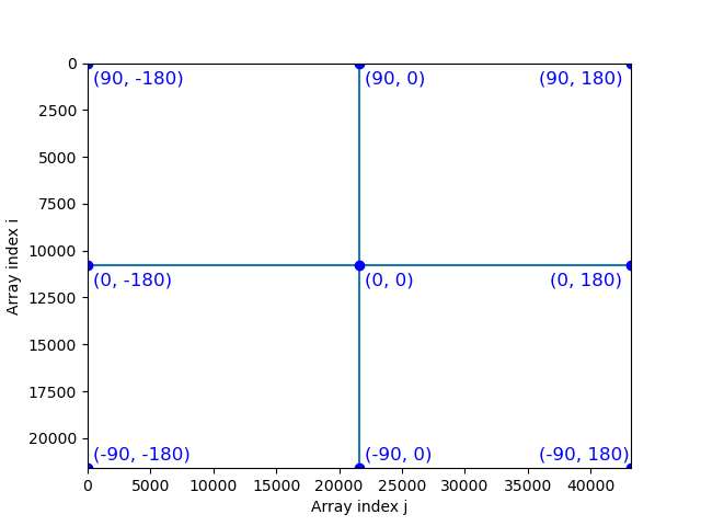
Let’s take the latitude / north-south / up-down direction first. We need a linear function that maps the latitude 90 to 0 and -90 to 21600.
Array indices need to be integers, so we truncate:
def lat_to_pixel(lat):
    return int(21600 * (90-lat) / 180)
The same for longitude / west-east / left-right. -180 should return pixel 0 and 180 should return 43200:
def lon_to_pixel(lon):
    return int(43200 * (lon-180) / 360)
Now we can write the function that replies with the landcover type at the requested spot:
def landcover_at_coord(lat, lon):
    i = lat_to_pixel(lat)
    j = lon_to_pixel(lon)
    return data[i,j]
Edge cases
It’s often easy to get the function working in 99% of all cases. But what about the edges? Exactly at latitude -90 our function returns 21600. But this is not a valid array index, the last valid index is 21599. We can fix this in different ways, but there’s no single right answer here.
We can make sure the highest index is 21599. The downside is that this shifts all the other pixel boundaries very slightly, too:
def lat_to_pixel__option_1(lat):
    return int(21599 * (90-lat) / 180)
My preferred option is a fixed pixel value for the problematic coordinate value:
def lat_to_pixel__option_2(lat):
    if lat == -90:
        return 21599
    else:
        return int(21600 * (90-lat) / 180)
This could now be extended to dealing with all sorts of nonsensical latitudes:
def lat_to_pixel(lat):
    if lat <= -90:
        return 21599
    elif lat > 90:
        return 0
    else:
        return int(21600 * (90-lat) / 180)
In the East-West direction things are a bit easier, since the coordinates actually
wrap around. We can treat -180 and +180 as the same place. The easiest way to fix that
is by using the modulus operation %. It gives us a cycling behaviour, for example:
[ (i % 4) for i in range(10) ]
gives us [0, 1, 2, 3, 0, 1, 2, 3, 0, 1]
Using the modulus for longitude keeps all return values between 0 and 43199:
def lon_to_pixel(lon):
    return int(43200 * (lon-180) / 360) % 43200
When we’re addressing edge cases in production code, it’s important to make consistent choices, and to document which choice has been made and why.
Finished program
The finished program also includes a little plot option,
to look at the area around the chosen point. The full code can be downloaded
at this link landcover_at_coord.py.
import numpy as np

data = np.memmap(
    'gl-latlong-1km-landcover.bsq',
    mode='r',
    dtype='uint8',
    shape=(21600, 43200),
)


landcover_names = { # r g b
0       : "Water",
1       : "Evergreen Needleleaf Forest",
2       : "Evergreen Broadleaf Forest",
3       : "Deciduous Needleleaf Forest",
4       : "Deciduous Broadleaf Forest",
5       : "Mixed Forest",
6       : "Woodland",
7       : "Wooded Grassland",
8       : "Closed Shrubland",
9       : "Open Shrubland",
10      : "Grassland",
11      : "Cropland",
12      : "Bare Ground",
13      : "Urban and Built",
}


def lat_to_pixel(lat):
    if lat <= -90:
        return 21599
    elif lat > 90:
        return 0
    else:
        return int(21600 * (90-lat) / 180)


def lon_to_pixel(lon):
    return int(43200 * (lon-180) / 360) % 43200


def landcover_at_coord(lat, lon):
    i = lat_to_pixel(lat)
    j = lon_to_pixel(lon)
    return data[i,j]


def main():
    while True:
        print('Enter q to quit')
        lat = input('Latitude (-90..90): ')
        if lat == 'q':
            break

        lon = input('Longitude (-180..180): ')
        if lon == 'q':
            break

        try:
            lat = float(lat)
            lon = float(lon)
        except ValueError:
            print('Not a decimal. Try again.')
            continue

        landcover_code = landcover_at_coord(lat,lon)
        landcover_name = landcover_names[landcover_code]

        print(f'The cover at {lat:.4f}, {lon:.4f} is {landcover_name}')

        #continue # always skip plotting

        show = input('Show plot? [y/n] ')
        if show == 'y':
            print('Close plot window to continue')
            show_plot(lat, lon)


def show_plot(lat,lon):
    import matplotlib.pyplot as plt
    from matplotlib import colors


    rgb_colors = np.array([
            ( 68,  79, 137),
            (  1, 100,   0),
            (  1, 130,   0),
            (151, 191,  71),
            (  2, 220,   0),
            (  0, 255,   0),
            (146, 174,  47),
            (220, 206,   0),
            (255, 173,   0),
            (255, 251, 195),
            (140,  72,   9),
            (247, 165, 255),
            (255, 199, 174),
            (  0, 255, 255),
    ])/255
    print(rgb_colors)
    landcover_cmap = colors.ListedColormap(rgb_colors)

    i = lat_to_pixel(lat)
    j = lon_to_pixel(lon)

    # radius of the plot area, 1px approx. 1km
    SIZE_px = 200
    SIZE_deg = SIZE_px/120

    imin = max(0, i-SIZE_px)
    imax = min(i+SIZE_px, 21599)

    jmin = max(0, j-SIZE_px)
    jmax = min(j+SIZE_px, 43199)

    latmin = max(-90, lat-SIZE_deg)
    latmax = min(lat+SIZE_deg, 90)

    lonmin = max(-180, lon-SIZE_deg)
    lonmax = min(lon+SIZE_deg, 180)

    plt.figure(figsize=(10,6))
    plt.title('UMD Global Land Cover Classification')
    plt.imshow(
        data[imin:imax, jmin:jmax],
        extent=(lonmin,lonmax,latmin,latmax),
        cmap=landcover_cmap,
        interpolation='none',
    )
    plt.xlabel('Longitude')
    plt.ylabel('Latitude')

    # draw the legend
    # https://stackoverflow.com/questions/40662475
    import matplotlib.patches as mpatches
    patches = [
        mpatches.Patch(color=rgb_colors[i], label=landcover_names[i])
        for i in range(len(landcover_names))
    ]
    plt.subplots_adjust(right=0.6)
    plt.legend(handles=patches, bbox_to_anchor=(1.05, 1), loc=2)

    plt.show()

if __name__ == '__main__':
    main()
References
- 1
Hansen, M., R. DeFries, J.R.G. Townshend, and R. Sohlberg (1998), UMD Global Land Cover Classification, 1 Kilometer, 1.0, Department of Geography, University of Maryland, College Park, Maryland, 1981-1994.
Hansen, M., R. DeFries, J.R.G. Townshend, and R. Sohlberg (2000), Global land cover classification at 1km resolution using a decision tree classifier, International Journal of Remote Sensing. 21: 1331-1365.