Pandas examples¶

Warning

Pandas is NOT part of the exam

Here we will take brief look at the Pandas library, using the example dataset we have used in the previous chapter.

Pandas is a very useful data analysis library, that makes many common tasks easy to handle. For all the detail, have a look at the introduction here:

Akvakultur¶

Load dataset¶

The data file is the same as before: ../csv/Akvakulturregisteret.csv.

The instructions on opening files tell us to use read_csv. The initial attempt

import pandas as pd
akva = pd.read_csv('Akvakulturregisteret.csv')
print(akva.columns)

fails with some errors. We need to tell it about the non-standard delimiter ; and text encoding iso-8859-1. Also, unusually, the header with column names is in row 1, not 0. Let’s provide all these as options:

import pandas as pd
import matplotlib.pyplot as plt

akva = pd.read_csv(
    'Akvakulturregisteret.csv',
    delimiter=';',
    encoding='iso-8859-1',
    header=1
)

print(akva.columns)
print(akva)

This looks like it works already. Compared to the CSV module, we have much more information in our pandas dataframe akva. The column names are automatically chosen, and I can print some information with e.g.:

print(akva['ART'])
print(akva['POSTSTED'].min(), akva['POSTSTED'].max())

Even slicing and filtering works like we’ve seen in numpy:

filter = akva['ART'] == 'Laks'
print(akva[filter])

Plotting¶

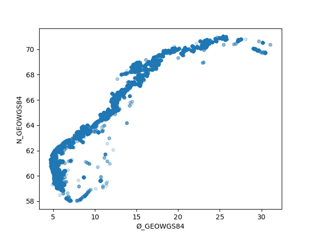
Let’s look at visualization. Again, the beginner tutorial on plotting is very informative. It looks like we only need to add another line, to see a scatterplot of all locations:

import pandas as pd
import matplotlib.pyplot as plt

akva = pd.read_csv(
    'Akvakulturregisteret.csv',
    delimiter=';',
    encoding='iso-8859-1',
    header=1,
)

print(akva)
print(akva.columns)

akva.plot.scatter(x='Ø_GEOWGS84', y='N_GEOWGS84', alpha=0.2)

plt.show()

Tasks from CSV chapter¶

The different common data analysis tasks we saw before can be done easily with pandas:

Count the different species (ART, column 12). Googling count categories in pandas suggested value_count():
```
print(akva['ART'].value_count())
```

Plot only those that grow Laks. Here, we can use filters:

laks = akva[ akva['ART'] == 'Laks' ]
laks.plot.scatter(x='Ø_GEOWGS84', y='N_GEOWGS84', alpha=0.2))

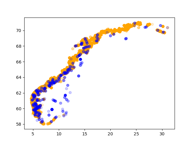
Plot FERSKVANN in one colour and SALTVANN in another (VANNMILJØ, column 20). Again we can use filters. The scatter plots here are the usual matplotlib plots, not the ones from pandas. You can see that the libraries work well with each other:

import pandas as pd
import matplotlib.pyplot as plt

akva = pd.read_csv(
    'Akvakulturregisteret.csv',
    delimiter=';',
    encoding='iso-8859-1',
    header=1,
)

salt = akva[ akva['VANNMILJØ'] == 'SALTVANN' ]
plt.scatter(x=salt['Ø_GEOWGS84'], y=salt['N_GEOWGS84'], c='orange', alpha=0.2)

fersk = akva[ akva['VANNMILJØ'] == 'FERSKVANN' ]
plt.scatter(x=fersk['Ø_GEOWGS84'], y=fersk['N_GEOWGS84'], c='blue', alpha=0.2)

plt.show()

Weather data¶

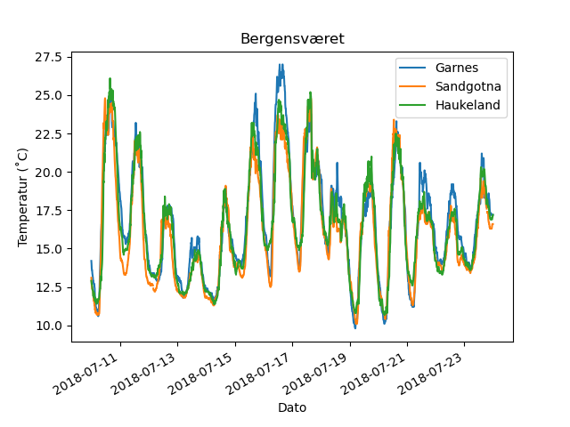
One of the strengths of Pandas is in analysing time series of measurements. Just to show what is possible, let’s take an example from https://www.bergensveret.no/ by UiB’s skolelab. These three data files contain weather data collected over 3 years, every 10 minutes.

Comparison¶

This code compares the three stations during July 2018:

import pandas as pd
import numpy as np
import pylab as plt

stations = [
"Garnes-2016-01-01-2019-09-16.csv",
"Haukeland-2016-01-01-2019-09-16.csv",
"Sandgotna-2016-01-01-2019-09-16.csv",
]

# loop over 3 files and read 3 dataframes
# into a list
dfs = []
for stn in stations:
    df = pd.read_csv(
            stn,
            index_col = 0,
            parse_dates = [0],
            na_values = '-9999',
            header = 0,
            names = [
                'dato','trykk','temperatur',
                'vindfart','vindretning',
                'fuktighet'
            ]
    )
    df['skole'] = stn.split('-')[0]
    dfs.append(df)

# combine all dataframes in the list into one dataset
weather = pd.concat(dfs)

skolene = ['Garnes','Sandgotna','Haukeland']
for skole in skolene:
    # choose two weeks in July 2018
    utvalg = weather[weather.skole==skole].loc['2018-07-10':'2018-07-23']
    #utvalg.temperatur.plot()
    utvalg['temperatur'].plot()

plt.legend(skolene)
plt.title('Bergensværet')
plt.ylabel('Temperatur (˚C)')
plt.xlabel('Dato')

plt.show()

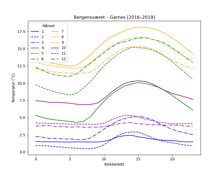
Grouping and averaging¶

We can also take one station and look at the average temperature during the day, for different months:

import pandas as pd
import pylab as plt

station = "Garnes-2016-01-01-2019-09-16.csv"

weather = pd.read_csv(
    station,
    index_col = 0,
    parse_dates = [0],
    na_values = '-9999',
    header = 0,
    names = [
        'dato','trykk','temperatur',
        'vindfart','vindretning',
        'fuktighet'
    ],
)

temp = weather.temperatur
# take the mean of all values in every month for every hour
grupper = temp.groupby([temp.index.month,temp.index.hour]).mean()

print(grupper)

# unstack level 0: use month as the different lines 
grupper.unstack(level=0).plot(
    style=['-','--','-.']*4,
    color=['blue']*3+['green']*3+['orange']*3+['purple']*3,
)
plt.title('Bergensværet – Garnes [2016–2019]')
plt.legend(title='Måned',ncol=2)
plt.xlabel('Klokkeslett')
plt.ylabel('Temperatur (˚C)')

plt.show()

Summary¶

Pandas is one of the most used data analysis tools in science, and offers far more than we can show in the frame of an introductory lecture on Python. If you find it useful, start on the pandas website, and follow through the tutorials with your own data in mind.